
In a previous article, we shared some reflections on machine learning models for data fitting and prediction, playing with a simple dataset related to the spread of the current coronavirus emergency. We looked at simple models and mentioned some more advanced ideas that rely upon deterministic dynamical system theory to be properly understood. However, that article was limited to so-called parametric models, which try to fit and predict data by using a known parametrized function with a fixed number of parameters.
Non-parametric models
For example, we considered an exponential function that transforms an input signal x into an output signal a exp(bx) with a, b parameters to be determined to best fit the training data. The merits of this approach are that it is simple to implement, since it requires only an optimizer, and there are usually very few parameters. Moreover, this is a white-box model: we know the function – after all, we chose it! – so we have plenty of theoretical tools available to justify its use, assess errors, and so on. We can also try to modify the function (as we did with the logistic example previously), with the knowledge, more or less, of what we are doing.
On the other hand, a non-parametric model is just a black box which accepts signal x and emits another signal – y – according to some inner rule that is dependent on numerous parameters hidden within the model, whose interpretation is largely unknown. We cannot modify the model and its parameters – usually much more numerous than in a parametric model – are tuned inside the black box. We have some external parameters (known as ‘hyper-parameters) that are within our control, but their tuning is totally empirical, since the black-box nature of the model means that we cannot even form hypotheses with any degree of certainty.
Put this way it seems that such models are difficult to deal with and frustrating to calibrate. That is undoubtedly true, but they are also often very effective, in some cases amazingly so. Most readers will already have guessed: artificial neural networks belong to this family of models.
In what follows we will play with some neural networks to analyse a simple dataset relating to the spread of COVID-19 in the state of New York, with the hope of gaining some insight into how these models should be applied and what can be expected from them. The Python snippets used below are by no means perfect, but nonetheless mediate between the use of library methods and, wherever possible, demonstrating what happens ‘behind the scenes’ by doing some computation by hand.
Neural networks come into play
As we will consider neural networks in the light of black boxes, to a certain extent we may ignore their inner structure and look at them as algorithms. These networks take a numeric input vector and provide another numeric vector as output, sometimes as minimal as a single number. In this case the network defines a function y = f(x1,…,xn), but notice that this function needs to be built based on a training set.
A training set contains data of the same format. For a function y = f(x1,…,xn), the training set is a set of pairs, called samples, (y1,(x11,…,x1n)),…,(ym,(xm1,…,xmn)) which are used to calibrate the function so that y1=f(x11,…,x1n),…,ym=f(xm1,…,xmn). Notice that numbers xij depend on two indexes: when dealing with neural networks be prepared to handle variables dependent on up to three indexes (improperly called tensors, even if we ignore their coordinate transformation rules).
A neural network has hidden parameters (called weights) which are changed each time a record of the training set fails an evaluation, in order to make corrections that enable the next evaluation to provide the desired result. Thus the network ‘learns’ the function values on the training set. More precisely, one might say say that the function has to fit the training set the best it can, and indeed neural networks can do this better than most other approximation and interpolation algorithms.
The function that our neural network should learn here is the curve of cases and/or the curve of deaths. However, it is not immediately able to do that, even though Neural networks are great at interpolating functions in order to fit known data and approximate unknown data. In our case, known data are all cases diagnosed up until the present day, while unknown data are all cases that will be diagnosed in the future. We are not interested in the curve between today and yesterday, so we are not interested in interpolating the curve but just in extrapolating from it.
Usually the function y = f(x1,…,xn) a neural network needs to interpolate depends on data which have no particular order: thus x1,…,xn are seen simply as coordinates of a point in some multi-dimensional space, and the proximity relationships (such as their distances) are taken into account. But when dealing with time series, time ordering is essential.
A ‘traditional’ neural network is just a set of parallel layers that contains the network nodes (called neurons), which in turn contain network weights. Neurons are connected so that information passes from one layer through to the next, starting from the input layer and ending with the output layer. The actual output is compared with the output expected from the training data, and weights inside nodes are adjusted by a rule called ‘backpropagation’ (or a variant thereof). After each layer-passing process is completed, weights are changed and their previous values are discarded, with the result that weights ‘have no memory’.
A class of neural networks called recurrent networks has been devised since the 1980s to deal with time series. In a recurrent network, some neurons are connected with themselves, consequently their output is also part of their input. This implies that these special networks ‘remember’ data that have previously passed through the network. This is an oversimplified and qualitative description but will suffice for our purposes. To learn more about this, read this excellent article by Stephen Grossberg on Scholarpedia.
There are several kinds of recurrent networks but the focus here is applying them to our problem in the form of black boxes. In order to do that we need to first deal with issues related to available data.
Setting up a recurrent LSTM network
As in the previous article of this series, I will use a time series maintained by The New York Times, with data based on reports from state and local health agencies (see this link).
from git import Repo
import matplotlib.pyplot as plt
import numpy as np
from os.path import join
from pandas import read_csv
from shutil import rmtree
from tempfile import mkdtemp

# Get data from github repository
tempdir = mkdtemp()
repo = Repo.clone_from("https://github.com/nytimes/covid-19-data", tempdir, branch="master", depth=1)
with open(join(tempdir, "us-states.csv")) as cf:
    DATA = read_csv(cf)
try:
    rmtree(tempdir)  # this may fail due to grant limitations...
except:
    pass

#Filter data we are interested in
NY_DATA = DATA.loc[DATA.state == "New York", ["cases", "deaths"]]
CASES = np.array(NY_DATA.loc[:, "cases"])
DEATHS = np.array(NY_DATA.loc[:, "deaths"])

# Plot the data
fig, axes = plt.subplots(2, 2, figsize=(10, 5))
axes[0,0].plot(CASES, "r+", label="Cases: data")
axes[0,1].plot(DEATHS, "k+", label="Deaths: data")
axes[0,0].legend()
axes[0,1].legend()
axes[1,0].hist(CASES)
axes[1,1].hist(DEATHS)Code language: PHP (php)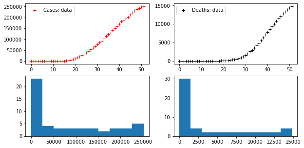
There are two time series provided with these data: the time series of COVID-19 cases (officially diagnised cases – a number usually far removed from the real number of cases and difficult to correlate to the true statistics) and the time series of deaths in which COVID-19 is the proven cause.
Since we want to use a neural network we need a training set. However, at the moment we only have a time series. If the aim is to predict, the time series may be used to provide a training set as follows: assume we have a time series s0,…,sN , being si numbers detected at times i=0,2,…,N. If we assume that the series is such that the next value depends only on the previous value (Markov hypothesis) then the prediction of si+1 is just a function of si, so the function that needs to be learnt is y = f(x) such that si+1 = f(si) for i = 0,…,N−1.
Therefore, our training data can be set up as (s1,s0),(s2,s1),…,(sN,sN−1). This can be done even if the output y is a vector rather than a single number. ‘Multivariate’ time series prediction is usually much harder than its ‘univariate’ equivalent, but this is not the case when using neural networks. In fact, there’s not much difference between the methods – both work in the same way – and in any case, the univariate option fits the purpose of this article.
Of course one could model more complex dependencies of the next value on those that precede it. For example, suppose we were to decide that the next value depended on the previous three values. In this situation, the function being modelled takes the form y = f(x1,x2,x3) and the training set becomes
(s3,(s0,s1,s2)),(s4,(s1,s2,s3)),…(sN,(sN−3,sN−2,sN−1))
The size of the input vector is called a step in this context. The previous example shows a three time-steps input, a one time-step output and a one step prediction. In general, the more steps used, the fewer samples can be arranged in the training set.
It is not difficult to write a code that will produce such samples from a single series. In the first example we will consider one time-step input. In the following script I download data and prepare training sets as previously described, plotting both series and their histograms.
# We use this function to produce training data with given input step (output step=1)
def extract_sample(series):
    X = []
    Y = []
    for i in range(len(series)-1):
        X.append(series[i:i+1])
        Y.append(series[i+1])
    return X, Y

# Training sets for both series: we separate input (x) from output (y) data
X_CASES, Y_CASES = extract_sample(CASES)
X_DEATHS, Y_DEATHS = extract_sample(DEATHS)Code language: PHP (php)
Now we have a training set, but we still need a model. There are many recurrent networks which may be used, but here we’ll use a classic model – the so-called LSTM (Long-Short Term Model). Dating back to 1997, this model is still a good choice in many cases (for example in natural language processing). The LTSM’s most striking feature is that some of the inner nodes of the network (nodes contain one or more weights) are used as network ‘memory’ rather than for computational purposes.
I won’t indulge in theoretical detail here, but will take the point of view of a developer and notice that this model is available for our use in the Keras Python library. In a momentit will be clear that taking this approach requires a bit of data preprocessing and the setting of a few parameters.
Let’s start with the simplest case – a one-layer LSTM. It is more or less straightforward to design the model using Keras API, setting some external parameters to standard values and setting hyper-parameters through trial and error. Such parameters include the number of nodes, the number of epochs and the batch size. The model is compiled by using the Keras backend – either Theano or TensorFlow – and can then be used to train data via the fit method. Eventually the model can be used (and tested) using the predict method.
We will use 80% of our sample as training samples, and the remaining data as test samples, and will concentrate on predicting deaths.
from keras.models import Sequential
from keras.layers import Dense
from keras.layers import LSTM

def train_test(neural_network, X, Y, epochs=5000, training_percent_size = 0.8):
    # This function takes a dataset, splits it into training and testing sets
    # according to training_percent_size, trains a plain LSTM model on it
    # launches preditions on datasets, and plots the result.
    N = len(X)
    # Extract training and testing samples and convert in numpy arrays
    n_training = int(N*training_percent_size)
    X_TRAINING, Y_TRAINING = np.array(X[:n_training]), np.array(Y[:n_training])
    X_TESTING, Y_TESTING = np.array(X[n_training:]), np.array(Y[n_training:])
    # neural_network.fit expect a (samples, input-steps, output-steps) shaped X array
    X_TRAINING = X_TRAINING.reshape((X_TRAINING.shape[0], X_TRAINING.shape[1], 1))
    X_TESTING = X_TESTING.reshape((X_TESTING.shape[0], X_TESTING.shape[1], 1))
    # Training: shuffle=False prevents data shuffling, order is important!
    for i in range(epochs):
        neural_network.fit(X_TRAINING, Y_TRAINING, epochs = 1, verbose = 0, shuffle = False)
        neural_network.reset_states()
    Y_PREDICTED = []    # we list predictions in this array
    for x in X_TESTING:
        x = x.reshape((1, 1, 1))
        y = neural_network.predict(x, verbose = 0)
        Y_PREDICTED.append(y[0][0])
    # Plot data in read and predictions in blue
    plt.plot(Y, 'r')
    plt.plot(range(n_training, N), Y_PREDICTED, 'b')
    plt.show()
    # Test loss
    print("Loss =", np.linalg.norm(Y_TESTING - np.array(Y_PREDICTED))**2/len(Y_TESTING))
    # The curve with prediction instead of testing values is returned
    return np.concatenate((Y_TRAINING, Y_PREDICTED))

# Set up the network with one layer of 10 nodes
nn = Sequential()
nn.add(LSTM(10, activation = "relu", input_shape = (1, 1)))
nn.add(Dense(1))   # the layer has a 1-dimensional output (a number!)
nn.compile(loss="mean_squared_error", optimizer="adam")

prediction = train_test(nn, X_DEATHS, Y_DEATHS)Code language: PHP (php)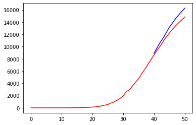
The result is not bad for a simple trial. At the very least, the model seems to follow the trend of the deaths curve.
To get a better result, the immediate impulse would be to add one more layer. Doing this with Keras is very simple, requiring just one more model.add instruction:
nn2 = Sequential()
nn2.add(LSTM(10, activation = "relu", input_shape = (1, 1), return_sequences=True))
nn2.add(LSTM(10, activation = "relu"))
nn2.add(Dense(1))  # the layer has a 1-dimensional output (a number!)
nn2.compile(loss="mean_squared_error", optimizer="adam")Code language: PHP (php)
In the previous snippet, the return_sequences=True option adjusts the output of the first layer to the input shape expected from the second layer, which is set to the same number of nodes as the first layer to keep things simple. The result is as follows:
prediction = train_test(nn2, X_DEATHS, Y_DEATHS)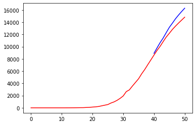
Inserting a new layer didn’t result in any significant improvement.
A bit of time series lore
Instead of blindly continuing in our attempts to improve our naive neural network, let’s try something a little cleverer. Those readers used to time series fitting will undoubtedly already be outraged by the poor pre-processing done in the above example. Time series are most effectively studied when they are paths of stationary processes – solutions of stochastic dynamical systems whose behaviour maintains, roughly speaking, mean and variance within a certain range. However, looking at our data, the trend of the curve clearly depends on time; there is no iterative structure at a first glance.
The good news is that, to some degree it is possible to transform a series into a stationary version, so that the transformation is invertible. The simplest way to do this is to look at the series of differences of the given series: s0,s1,…,sN, thus
d1 = s1 − s0, d2 = s2 − s1, …, dN = sN − sN−1
In both cases, the transformation (s1,…,sN) → (d1,…,dN) is invertible (notice that we excluded s0 from the original series, kept aside as a sort of ‘initial condition’), and the inverse is given by the recursive relationship:
s1 = s0 + d1, s2 = s1 + d2, …, sN = sN−1 + dN
In some sense the original series is the cumulative series of the series of differences. Another option would be to define a difference series with a given step k:
dk = sk − s0, dk+1 = sk+1 − s1, …, dN = sN − sN−k
Let us try our two coronavirus series with step k=1:
def difference(s):
    return [s[i+1] - s[i] for i in range(len(s)-1)]

def cumulated(s0, d):
    # cumulated(s[0], difference(s)) == s
    s = [s0]
    for i in range(len(d)):
        s.append(s[i] + d[i])
    return s

D_CASES = difference(CASES)
D_DEATHS = difference(DEATHS)

fig, axes = plt.subplots(2, 2, figsize=(10, 5))
axes[0,0].plot(D_CASES, "r+", label="Cases diff")
axes[0,1].plot(D_DEATHS, "k+", label="Deaths diff")
axes[0,0].legend()
axes[0,1].legend()
axes[1,0].hist(D_CASES)
axes[1,1].hist(D_DEATHS)Code language: PHP (php)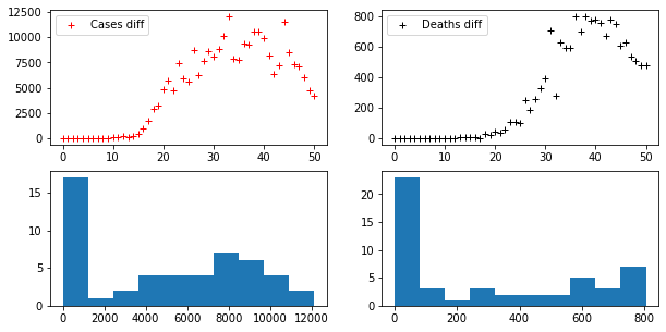
Differentiation may be iterated, thus we may consider a second difference of the series (the series that expresses the difference of its difference), and so on. At each step the series become more and more similar to a stationary series. Of course, the k-th difference of a given series has k elements fewer than the original one.
For example let us compute the third difference of our series:
D3_CASES = difference(difference(difference(CASES)))
D3_DEATHS = difference(difference(difference(DEATHS)))

fig, axes = plt.subplots(2, 2, figsize=(10, 8))
axes[0,0].plot(D3_CASES, "r+", label="Cases diff^3")
axes[0,1].plot(D3_DEATHS, "k+", label="Deaths diff^3")
axes[0,0].legend()
axes[0,1].legend()
axes[1,0].hist(D3_CASES)
axes[1,1].hist(D3_DEATHS)Code language: JavaScript (javascript)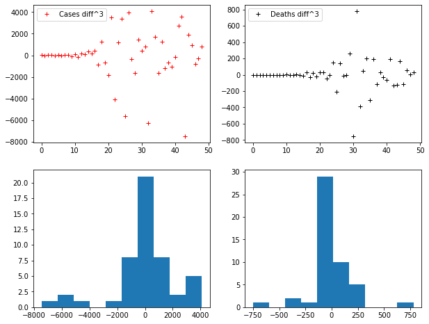
Notice that the histograms tend to become more and more similar to normal distributions.
Next, we will again perform the training of the neural network on differentiated data, and convert the results back into cumulative form. This performance produces an impressive improvement:
plt.figure(0)
DX_DEATHS, DY_DEATHS = extract_sample(D_DEATHS)
d_prediction = train_test(nn2, DX_DEATHS, DY_DEATHS)

# We plot also the actual series
plt.figure(1)
prediction = cumulated(Y_DEATHS[0], d_prediction)
plt.plot(prediction, 'b')
plt.plot(Y_DEATHS, 'r')
print("Loss =", np.linalg.norm(Y_DEATHS - np.array(prediction))**2/len(Y_DEATHS))Code language: PHP (php)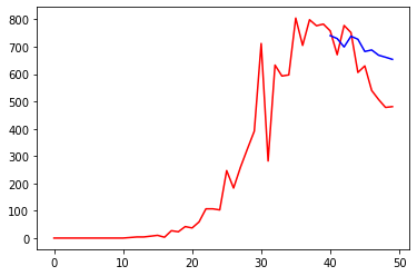

Another invertible transformation that it makes sense to apply to our case studies is the scaling transformation, by means of which we reduce our data to within a fixed interval. When using neural networks this is a worthwhile path to pursue, as such networks have nodes that usually output numbers between -1 and 1, unless otherwise stated. For example, one could use the ‘relu’ activation function, popular in deep learning, which cuts negative values.
The ‘relu’ specification may be dropped, but the data has to be rescaled. First, here is a demonstration of the scaling function, which simply takes the minimum and maximum value of the series and linearly transforms the former into -1 and the latter into 1 (and all numbers in between accordingly). This scaling is applied to the difference series:
def scaling(s, a = -1, b = 1):
    m = min(s)
    M = max(s)
    scale = (b - a)/(M - m)
    return a + scale * (s - m)

DS_CASES = scaling(difference(CASES))
DS_DEATHS = scaling(difference(DEATHS))

fig, axes = plt.subplots(1, 2, figsize=(10, 4))
axes[0].plot(DS_CASES, "r+", label="Cases diff+scaled")
axes[1].plot(DS_DEATHS, "k+", label="Deaths diff+scaled")
axes[0].legend()
axes[1].legend()Code language: JavaScript (javascript)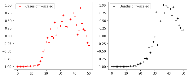
Finally, let us check our basic LSTM network on these data, and transform the results back again to provide a prediction as we did previously. The same parameters are used to train the network, but the activation function is left as the default, which is a sigmoid function between -1 and 1.
nn3 = Sequential()
nn3.add(LSTM(10, input_shape = (1, 1), return_sequences=True))
nn3.add(LSTM(10))
nn3.add(Dense(1))  # the layer has a 1-dimensional output (a number!)
nn3.compile(loss="mean_squared_error", optimizer="adam")

plt.figure(0)
DSX_DEATHS, DSY_DEATHS = extract_sample(DS_DEATHS)
ds_prediction = train_test(nn3, DSX_DEATHS, DSY_DEATHS)

# We plot also the actual series
plt.figure(1)
d_prediction = scaling(ds_prediction, min(D_DEATHS), max(D_DEATHS))
prediction = cumulated(Y_DEATHS[0], d_prediction)
plt.plot(prediction, 'b')
plt.plot(Y_DEATHS, 'r')
print("Loss =", np.linalg.norm(Y_DEATHS - np.array(prediction))**2/len(Y_DEATHS))Code language: PHP (php)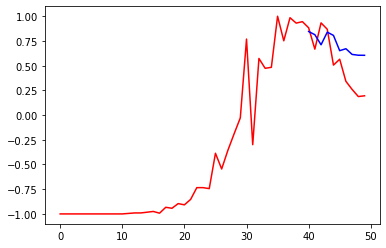
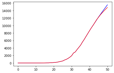
Another improvement is obvious: our predictions are far from being reliable in the long term but give quite a reasonable approximation of the curve related to deaths.
Conclusions
In this article we set up a simple non-parametric model to predict time series, and applied it to data on the spread of COVID-19. The techniques demonstrated here can be greatly improved on in several respects – by using stateful LSTM models, for example, and also by using different and more informative datasets.
However, the aims of this article were:
- To point out the differences between the parametric(more math, specific domain considerations, etc.) and non-parametric models (framework use, guessing hyper-parameters, etc.).
- To show how data preparation not a trivial task in machine learning algorithm implementation. Most of the code written here was the product of data handling, while the model was set up in a handful of API calls.
- To point out that simply making a more complicated neural network does not imply a corresponding gain in performance. It is very easy to complicate the model in Keras, but this should be done only if actually needed. Experiment by changing hyper-parameters to find a good combination rather than by adding layers.
- To stress the importance of knowing what we are doing. Starting with some elementary techniques for time series, we improved the result by simply transforming the input data, without making any changes to the model!
Above all, human reflection about machine algorithms is always needed. Leaving relevant choices to the data scientists who design and implement the simulation remains the key to understanding a real phenomenon (such as viral spread).
If you are interested in these topics, do not miss the opportunity to attend our Deep Learning online conference: click here for more information!


