The life of a developer nowadays is a very exciting one: we have several languages, frameworks, and numerous excellent tools available to select from according to our needs.
Not only that, we also have a lot of interesting and useful techniques that have been developed to allow us to accomplish purposes far beyond the traditional business– or science-oriented computations demanded of programmer-developed programs.
For example, in our Web applications we want nice responsive GUIs, integration with identity and access management systems, no SQL databases to properly store unstructured data downloaded from the Internet, etc. etc.
Time and again, our customers require a class of techniques and algorithms relating to Artificial Intelligence (AI). From games to search engines, from service desks to e-commerce sites, AI seems to be ubiquitous and a necessary tool for any developer to know, or better still, know how to use.
Not surprisingly, artificial intelligence will be one of the main topics covered at the upcoming Codemotion Online Tech Conference on October 2020: check the agenda and get your free ticket at this link!
And, if you want to know more about how modern technologies and tools can support you for – and during – the organisation of a virtual event, don’t miss this article showcasing the best tools we used to host our online conferences since the COVID-19 outbreak.
However, it is worth noting that the equation AI = ML (machine learning) = ANN (artificial neural networks) is definitely false: AI is a broader field than ML, and ML involves many algorithms unrelated to neural networks. A particularly interesting class of such algorithms are evolutionary algorithms.
Learning as evolving
As neural networks, which draw inspiration from an oversimplified model of the human brain, evolutionary algorithms are inspired by biology – not from individual physiology, but rather from species behaviour. The most basic clusters of living creatures, species evolve to adapt to a changing environment.
The evolutionary process uses random errors in DNA copying when individuals reproduce to originate new features in individuals. These new features allow said individuals to live more successfully in the changed conditions of their environment.
Roughly speaking, and oversimplifying somewhat, the basic features of evolution in biological systems are:
- Individuals of a species live in a changing environment.
- Only a fraction of individuals reach adult age and reproduce.
- Individuals are formed (in a complex way) by their genetic code.
- Individuals compete to reproduce.
- During reproduction, both gene recombination and genetic mutation occur.
- Individuals displaying mutated characteristics experience natural selection due to their evolving fitness for the environmental conditions.
The idea of evolutionary algorithms is to use the process of individual mutation and species evolution as an iterative optimization algorithm. The ultimate goal of such an algorithm is to determine the individual most fitted for a certain environment.
Of course, algorithms do not deal with living creatures; their ‘individuals’ are objects upon which a certain fitness function may be computed.
Therefore, evolutionary algorithms allow possible solutions of a single problem to compete and recombine so as to produce new solutions. From these new solutions, the most improved are selected, and the process continues until the optimal solution is found.
Evolutionary algorithms should be considered machine learning algorithms as they learn the optimal solution by iteration and trials: they do not need a training set, but work on the structure of the possible solutions by randomly making changes according to the response of the environment. This is a fitness function that ranks the computed solutions according to how optimal they are.
In short, evolutionary algorithms learn by enforcing the evolution of data that represents solutions to optimization problems (a neural network also evolves its weights in a sense, using the backpropagation algorithm, but it needs several sets of training data to arrive at the solution to the problem).
Convergence in revolutionary algorythms
There are various interesting theories regarding convergence in evolutionary algorithms, but these are of no concern to us here. Our interest is in understanding how these algorithms may be used to solve Artificial Intelligence problems, rather than in understanding why they actually work (although it is important to stress that there is a lot of theoretical work in analysing the properties of evolutionary algorithms, unlike when dealing with neural networks).
One important class of evolutionary algorithms used in practical applications is genetic algorithms: these stress the importance of the data representation used to encode possible solutions to our optimization problem.
The class name is inspired by an analogy with genetic code – the material that encodes (in a very complex way) our ‘phenotype’ or physical appearance. The use of the adjective ‘genetic’ reflects the fact that evolving solutions are represented by data structures, usually strings, reminiscent of biological genetic code.
Since the terminology in this field is borrowed from genetics, let us clarify some definitions for these terms used in the context of computing:
- phenotype is a possible solution to our optimization problem.
- chromosome is a data structure which completely encodes a phenotype (in biological systems several chromosomes correspond to a phenotype, in genetic algorithms the correspondence is 1-1).
- population is a set of chromosomes.
- generation is a population at a certain time.
- fitness is a function which measures how optimal a phenotype is for the goal.
- evaluation is the process of getting a phenotype from a chromosome to apply the fitness function to it.
The goal of a genetic algorithm
The goal of a genetic algorithm is to discover a phenotype that maximises fitness, by allowing a certain population to evolve across several generations.
The next question is: how does the evolution of individuals happen? Genetic algorithms apply a set of ‘genetic operations’ to chromosomes of each generation to allow them to reproduce and, in the process, introduce casual mutations, much as occurs in most living beings.
The process which allows individuals to reproduce is the crossover operator; this takes two chromosomes, which are data structures, and produces two new chromosomes. These new chromosomes are obtained by splitting each original chromosome into two pieces and recombining these.
For example, supposing the chromosomes to be bytes: if we have c1 = |01001010| and c2 = |11010101|, then we may choose to crossover them by splitting them into two nibbles (a.k.a. 4-bits) and recombine them in one of two possible ways:
|0100|0101|(the first nibble ofc1concatenated with the second nibble ofc2)|1101|1010|(the first nibble ofc2concatenated with the second nibble ofc1)
Here, we are cut/pasting chromosomes at their mid-point, but we could choose to cut elsewhere, or even to cut at more points. The same process could be carried out with character strings or arrays.
Crossover takes place between individuals of a generation to produce the next generation. However, not all individuals reproduce; instead (as readers will surely know from many wildlife documentaries) only the best-adapted individuals have that opportunity.
Similarly, crossover is used in genetic algorithms only between certain individuals, chosen from among those best fitted (although variants of these algorithms of course require that all individuals should reproduce).
A typical measure of the fitness needed to reproduce is to compute, for each individual x, the probability
p(x) = Fitness of x / sum of fitness of all individuals
the individuals for which the probability is highest are then chosen.
The mutation operator introduces randomness into the crossover; this operator randomly changes one or more elements of the chromosome. For example, one can choose to mutate two bits in a byte following each crossover. Usually the mutation rate is low.
Now we can write down the general scheme of a genetic algorithm: we should have
- a fitness function F(x) which may be applied to a phenotype;
- a threshold F_T such that if F(x) ≥ F_T then x is considered to be an optimal solution for our problem;
- the number N of individuals in our population (remember: individuals, phenotypes and chromosomes are in 1-1 correspondence);
- the number 0≤ r ≤ 1 of individuals in a generation which will be replaced by crossover-generated individuals;
- the mutation rate 0 ≤ m ≤ 1.
Then the algorithm runs as follows:
Initialize the population generation to N random chromosomes.
While max(F(x) for x in generation) < F_T:
    Initialize a new empty population next_generation
    For each x in generation:
    compute s[x] = F(x) / sum(F(y) for y in generation)
    Insert into next_generation the (1-r)*N chromosomes from generation
    which have highest scores s[x]
    Select r*N/2 individuals (with highest score) from generation
    and let them reproduce by crossover, adding the two offsprings
    to next_generation.
    Select at random m*N individuals from next_generation and mutate
    their chromosomes.
    Let generation = next_generationCode language: JavaScript (javascript)
Note that a new population is produced; this will be the next generation, into which we insert the best-adapted individuals of the current generation, and their offspring. The resulting (next) generation is the same size as the previous generation.
It is worth stressing that such an algorithm is an iterative algorithm in which a series of parameters change at each iteration (the chromosomes), and which is governed by certain hyper-parameters such as numbers r and m. Namely, a typical machine learning algorithm.
The previous algorithm is almost Python-esque in its coding, so it’s impossible to resist implementing it in a working program to play with. We’ll use this to solve a simple regression problem with genetic algorithms.
How to implement genetic algorithms in Python
Let us try to implement a simple evolutionary algorithm: suppose we have N data to fit, y1,…,yN, for example N numbers which represent measurements of a certain variable at given instants: temperatures, house prices, etc. For simplicity, let us assume that instants t1,t2…,tN at which our measurements were taken are 0,1,…,N−1.
We want to find a curve that fits the data, i.e., we want to interpolate it.
There are several classic methods of achieving that which do not require machine learning (although neural networks may be efficiently used for that purpose), for example Lagrange interpolation: the latter finds a polynomial of degree N, thus a function of the form p(x) = a0 + a1 x + a2 x2 + … + aN xN to achieve the desired outcome.
To crossover polynomials is a difficult matter (even if polynomials can easily be represented as arrays (a0, a1, …, aN)), so we will stick to simpler functions, e.g., piecewise linear functions.
Such a function is simply a joining of segments along vertices, as in the following graph:
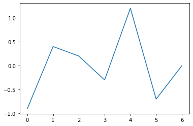
A piecewise linear function is determined by the set of its vertices, which are points (x,y) in the Cartesian plane. In our case, the vertices are (t0, p0), (t1, p1), …, (tN, pN) (I use pi to suggest ‘piecewise’).
We will use an evolutionary algorithm, trying to fit N points into such a piecewise linear function: a function of this sort is determined by its values [p0, p1, …, pN], so, as developers would say, it is just an array of numbers with N+1 elements.
In the genetic algorithm parlance introduced above:
- a piecewise linear function is a phenotype;
- its vector encoding is a chromosome;
- the fitting function takes the piecewise linear function p(t) corresponding to a chromosome, evaluates it at points t0, …, tN, which is essentially just considering the vector (p0, …, pN), and comparing it with the vector (y0, …, yN), for example by taking the norm of their difference. The more optimal the solution, the smaller the latter will be, so we will take its inverse (C −∥p − y∥)/C as the fitting function for C.
Notice once again that a phenotype is represented by a chromosome; in this case the phenotype is a function but the chromosome is a fixed length vector.
We’ll artificially produce the points we want to fit, so that they are on a damped sinusoid:
import matplotlib.pyplot as plt
import numpy as np
from numpy.random import randint, uniform

# Points to fit
n_points = 15
times = np.linspace(0, 12, num = n_points)
points = np.array(np.exp(-0.2*times)*(np.cos(times)))
finer = np.linspace(0,12)
plt.plot(finer,np.array(np.exp(-0.2*finer)*(np.cos(finer))))
plt.show()Code language: PHP (php)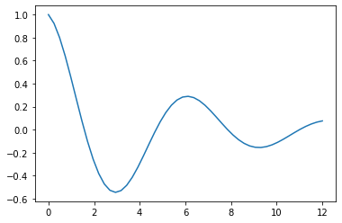
As usual, our implementation of the previous algorithm will be very simple and will demand as little as possible of our language (Python) so as to be easily understandable and portable. An appropriate alternative would be to define a class GA to perform our algorithm, however we will stick to a script-like program here.
In our first code snippet we set hyper-parameters, initialize the population and plot the piecewise linear function corresponding to selected chromosomes.
# Hyper parameters
N = 50
d = n_points
r = 0.7    # percentage of chromosomes to crossover
m = 0.1    # percentage of chromosomes to mutate

# The current generation (which is formed by chromosomes)
generation = np.random.uniform(-2, 2, (N, d))

def Fitness(i):
    """Fitness function for chromosome i: the higher the function,
        the better the phenotype fits the goal."""
    return (1000 - np.linalg.norm(generation[i,:] - points)) / 1000

FT = 0.999   # If Fitness > FT we have an optimal solution

# Prints some phenotypes corresponding to initial population
plt.plot(times, generation[0])
plt.plot(times, generation[1])
plt.plot(times, generation[2])
plt.show()Code language: PHP (php)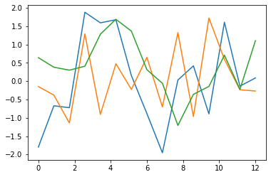
Note that the fitness function should be higher for piecewise functions that are nearer to the function to fit. We use the norm of the difference of two vectors (the values of functions compared at fixed points) but we complement and normalize it between 0 and 1 to get a fitness function which is closer to 1 the more the piecewise function approximates the function to fit.
Now, we implement the genetic algorithm by translating the pseudocode used above into Python: we define the crossover function with a simple standard operator used for chromosomes made of arrays of real numbers.
Moreover, note that we compute scores and use them as probability, or better yet, as a probability distribution from which to draw samples.
To do that we define a vector of indexes, which contains copies of the same index j according to the score of generator[j] and then choose an index uniformly from this vector, simulating the non-uniform drawing from the empirical distribution created by the scores.
Finally, mutations simply add a random number between -1 and 1 to the real numbers of the chromosome to be mutated: mutations are needed to explore new regions in the space state of the solutions to the problem, and to introduce a stochastic global search feature in the genetic algorithm.
def crossover(j1, j2):
    """Cross over generation[j1] and generation[j2]. For each gene of the
       Chromosome we take the max and min of the corresponding genes in j1 and
       j2 and set the offspring coordinates to a random number in the interval
       [min, max] """
    offspring1 = []
    offspring2 = []
    for i in range(d):
        m = min(generation[j1,i], generation[j2,i])
        M = max(generation[j1,i], generation[j2,i])
        offspring1.append(np.random.uniform(m, M))
        offspring2.append(np.random.uniform(m, M))
    return offspring1, offspring2

def scores():
    """Returns the vector of scores of the current generation"""
    s = []  # array of scores
    for j in range(N):
        s.append(Fitness(j) / sum(Fitness(k) for k in range(N)))
    return s

max_iterations = 1000
while max_iterations > 0 and max(Fitness(i) for i in range(N)) < FT:
    # decreases the loop counter
    max_iterations -= 1

    #Initialize a new empty population next_generation
    next_generation = np.zeros((N, d))

    # For each x in generation compute s[x]=F(x)/sum(F(y) for y in generation)
    s = scores()

    # Now create a vector of indexes where the most probable indexes (the one
    # with highest scores) are repeated more than others.
    v = []
    for j in range(N):
        v.extend([j] * int(N*s[j]))
    # Thus, if we choose uniformly random elements from v is like to draw from
    # the probabilistic distribution induced by probabilities s[j]

    # Insert into next_generation the (1-r)*N chromosomes from generation by
    # drawing from distribution s[].
    j = 0
    while j < int(N*(1-r)):
        k = v[np.random.randint(len(v))]
        next_generation[j] = generation[k]
        j += 1
    # Select r*N/2 individuals (with highest score) from generation and let them
    # reproduce by crossover, adding the two offsprings to next_generation.
    for k in range(int(r*N/2)):
        # Select a pair (j1, j2) of individuals to reproduce
        j1 = v[np.random.randint(len(v))]
        j2 = v[np.random.randint(len(v))]
        while j1 == j2:
            j2 = v[np.random.randint(len(v))]
        offspring1, offspring2 = crossover(j1, j2)
        next_generation[j,:] = offspring1
        next_generation[j+1,:] = offspring1
        j += 2

    # Select at random m*N individuals from next_generation and mutate their
    # chromosomes.
    for j in range(int(m*N)):
        j1 = v[np.random.randint(len(v))]
        for k in range(d):
            next_generation[j1,k] += np.random.uniform(-1,1)

    generation = next_generationCode language: PHP (php)
Let us plot the solution found by the algorithm: it is of course a piecewise linear function, so it cannot have the smooth appearance of the function to fit, but it does mimic the function’s increase and decrease trends, giving at the very least a qualitative idea of the function.
# Plots the optimal solution
i_optimal = np.argmax(scores())
plt.title("Optimal solution")
plt.plot(times, generation[i_optimal])
plt.plot(np.linspace(0,12), np.array(np.exp(-0.2*np.linspace(0,12))*(np.cos(np.linspace(0,12)))))
plt.show()Code language: PHP (php)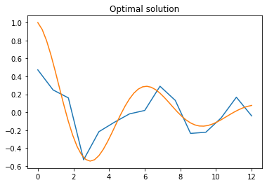
Of course, as is usual for machine learning algorithms, hyper-parameters may be fine tuned to improve the result, but for the sake of our expository discussion we can leave that to the reader to play with.
Notice that if r = 0 then no crossover occurs, while if m = 0 no mutations occur: one can play with these numbers to see how the algorithm behaves with these extreme values. The crossover function may also be changed in several respects, but the main ingredients of genetic algorithms have been displayed in this test example.
Want to launch a developer event despite the challenges of COVID-19?
If you want to know more about how modern technologies and tools can support you for – and during – the organisation of a virtual event, don’t miss this article showcasing the best tools we used to host our online conferences since the COVID-19 outbreak.

